Introduction

The note is based on a MIT open course by professor Gilbert Strang. The note is to alter my perspective on matrices and spaces. Hopefully, at then end of the post, I will have some more insights in linear algebra, an essential subject for statistical algorithms.

Contents

1. Matrices
2. Spaces
3. Projections
4. Orthogonality
5. Determinants
6. Eigenvalues & Eigenvectors

Matrices

Intro to Matrices

Let us say there are two linear equations,

\[\begin{aligned} 2x-y&=0\\ -x+2y&=3\\ \leftrightarrow\\ \begin{bmatrix} 2&-1\\-1&2 \end{bmatrix}\begin{bmatrix} x\\y \end{bmatrix}&=\begin{bmatrix} 0\\3 \end{bmatrix} \end{aligned}\]

There are several ways to view this and one way would be by row picture which would plotting a 2-D plane graph with the top two linear equations (we’re quite experienced with this). However, we can also see this by column picture.

\[\begin{aligned} x\begin{bmatrix} 2\\-1 \end{bmatrix}+y\begin{bmatrix} -1\\2 \end{bmatrix}&=\begin{bmatrix} 0\\3 \end{bmatrix} \end{aligned}\]

This picture can be illustrated into another 2-D plot with vectors. This equation is called the linear combination of columns and is often denoted as \(A\boldsymbol{x}=\boldsymbol{b}\).

It doesn’t seem so different when there are two equations, but when we think of situations with 3 equations, it is a lot more easier to think of a plot with 3 vectors (column picture) than 3 plane collision (row picture).

Coming back to the 2 equations, can we solve \(A\boldsymbol{x}=\boldsymbol{b}\) for every \(\boldsymbol{b}\)? The question can be translated into two different perspectives. From the perspective of “row”, will there going to be every solution for every \(\boldsymbol{b}\)? From the perspective of “column”, do the linear combination of the columns fill 2-D space? If the two columns lie on the same plane, the answer would be no.

\[\begin{aligned} A=\begin{bmatrix} 1&-2\\2&-4 \end{bmatrix} \end{aligned}\]

The column picture allows us to see the linear equations into a combination of vectors which gives us a clear way to observe.

Elimination

Let us say there are 3 equations,

\[\begin{aligned} x+2y+z&=2\\ 3x+8y+z&=12\\ 4y+z&=2\\ \leftrightarrow \\ \begin{bmatrix} 1&2&1\\3&8&1\\0&4&1 \end{bmatrix}\begin{bmatrix} x\\y\\z \end{bmatrix}&=\begin{bmatrix} 2\\12\\2 \end{bmatrix} \end{aligned}\]

It is really difficult to plot vectors in head once the dimension eleveates. So humans have found out a way to solve linear equations by elimination.

\[\begin{aligned} x+2y+z&=2\\ 3x+8y+z&=12\\ 4y+z&=2\\ \leftrightarrow\\ 3x+6y+3z&=6\\ 3x+8y+z&=12\\ 4y+z&=2\\ \leftrightarrow\\ -2y+2z&=-6\\ 4y+z&=2\\ \leftrightarrow\\ z&=-5\\ y&=\frac{7}{4}\\ x&=1 \end{aligned}\]

This is also possible with the matrix augmenting the b column.

\[\begin{aligned} [A|\boldsymbol{b}]=\\ \ \\ \begin{bmatrix} \ldots row1 \ldots\\\ldots row2 \ldots\\\ldots row3 \ldots \end{bmatrix}&=\\ \ \\ \begin{bmatrix} 1&2&1&2\\3&8&1&12\\0&4&1&2 \end{bmatrix} \rightarrow\begin{bmatrix} 1&2&1&2\\0&2&-2&6\\0&4&1&2 \end{bmatrix} &\rightarrow\begin{bmatrix} 1&2&1&2\\0&2&-2&6\\0&0&5&-10 \end{bmatrix}\\ \ \\ =[U\boldsymbol{c}] \end{aligned}\]

The last part is to seperate the matrix and the column and solve \(U\boldsymbol{x}=\boldsymbol{c}\). However, there must be something more than just arrows when transforming. If we focus on the first arrow, we are executing “subtract 3 row1 from row2” to turn (2,1) element into 0. And since (3,1) element is 0, we skip to the next step where we want to “subtract 2 row2 from row3” to turn (3,2) element into 0.

\[\begin{aligned} E_{21}A&=\begin{bmatrix} \ & r_1 & \ \\ \ & r_2 & \ \\ \ & r_3 & \ \\ \end{bmatrix}\begin{bmatrix} 1&2&1\\3&8&1\\0&4&1 \end{bmatrix}=\begin{bmatrix} 1&2&1\\0&2&-2\\0&4&1 \end{bmatrix}\\ \leftrightarrow\\ E_{21}&=\begin{bmatrix} 1&0&0\\-3&1&0\\0&0&1 \end{bmatrix} \end{aligned}\]

Before trying to understand the mechanism hiding here, we need to understand the matrix multiplication.

4 Types of Matrix Multiplication

We will skip the dot product (row times column) part because it is a very simple process.

\[\begin{aligned} AB=C\\ \leftrightarrow\begin{bmatrix} \ & \ & \ \\ c_1 & c_2 & c_3 \\ \ & \ & \ \\ \end{bmatrix}\begin{bmatrix} \ & r_1 & \ \\ \ & r_2 & \ \\ \ & r_3 & \ \\ \end{bmatrix}\ldots(1)\\ \begin{bmatrix} \ & \ & \ \\ \ & A & \ \\ \ & \ & \ \\ \end{bmatrix}\begin{bmatrix} \ & \ & \ \\ c_1 & c_2 & c_3 \\ \ & \ & \ \\ \end{bmatrix}\ldots(2)\\ =\begin{bmatrix} \ & r_1 & \ \\ \ & r_2 & \ \\ \ & r_3 & \ \\ \end{bmatrix}\begin{bmatrix} \ & \ & \ \\ \ & B & \ \\ \ & \ & \ \\ \end{bmatrix}\ldots(3)\\ =\begin{bmatrix} \ & \ & \ \\ \ & C & \ \\ \ & \ & \ \\ \end{bmatrix}\\ \end{aligned}\]

(1) is the outer product (column times row). Each of the multiplication of column and row is a matrix and the sum adds up to become C. (2) illustrates that the columns of C is the combination of columns of B\(A\times col_k^B=col_k^C\). (3) shows that the row of C is the combination of rows of A \(row_k^A\times B=row_k^C\). (2) and (3) can be organized as following; column operation for (2), row operation for (3). Implementing this to the previous example, in order to operate by rows in the right side of the equation, we need to multiply a matrix on the left. If you can’t see it right away, try (3) and (1) in order.

\[\begin{aligned} \text{(Ex 1)}\\ E_{21}A&=\begin{bmatrix} \ & r_1 & \ \\ \ & r_2 & \ \\ \ & r_3 & \ \\ \end{bmatrix}\begin{bmatrix} 1&2&1\\3&8&1\\0&4&1 \end{bmatrix}=\begin{bmatrix} 1&2&1\\0&2&-2\\0&4&1 \end{bmatrix}\\ \ \\ r_1A&= first\ row\ of\ A \\ r_2A&= second\ row\ - 3\ first\ row\ of\ A\\ r_3A&= third\ row\ of\ A \\ E_{21}&=\begin{bmatrix} 1&0&0\\-3&1&0\\0&0&1 \end{bmatrix}\\ &E_{32}E_{31}(E_{21}A)=U\\ &E_{32}E_{31}(E_{21}[A|\boldsymbol{b}])=[U|\boldsymbol{c}]\\ \end{aligned}\]

So, if we are trying to operate by columns in the right side of the equation, we need to multiply a matrix on the right. This leads to the answer why the equation below is true.

\[\begin{aligned} AB \neq BA \end{aligned}\]

In addition, what the E matrices; elementary matrices are really doing is just applying multiplication + subtraction between rows. Therefore, we can infer there is some multiplication that would do the operation backwards; inverse.
\(\begin{aligned} &U\rightarrow A\\ &?U=A \end{aligned}\)

• Bonus: What if we there are times we need both row and column operation? Is there an order for it?

  No. \(\begin{aligned} E_rBE_c = (E_rB)E_c = E_r(BE_c) \end{aligned}\)

• Bonus 2: What if the second pivot is 0 after the E(2,1) progress?

  \[\begin{aligned} \begin{bmatrix} 1&2&1\\3&6&1\\0&4&1 \end{bmatrix}\rightarrow\begin{bmatrix} 1&2&1\\0&0&-2\\0&4&1 \end{bmatrix} \end{aligned}\]

  We can exchange the row 2 and 3; permutation.

Inverse

So, we want a matrix that does exactly backwards what it does. If the matrix does its operation -> do it backwards, it is going to do nothing on the target matrix; identity matrix. It returns the exact matrix as you can see by thinking of the three types of multiplication from prior section.

\[\begin{aligned} I=\begin{bmatrix} 1&0\\0&1 \end{bmatrix} \end{aligned}\]

So,

\[\begin{aligned} A^{-1}A &= AA^{-1} = I\\ \leftrightarrow E[A|I] &=[I|A^{-1}]\\ \leftrightarrow E&=A^{-1} \end{aligned}\]

Just like the prior section (Ex 1), A is going to be manipulated by E into I. Coming back to the elimination, when we say there is no situation such as ‘Bonus2’,

\[\begin{aligned} &E_{32}E_{31}E_{21}A = U\\ &\leftrightarrow\\ &A = E_{32}^{-1}E_{31}^{-1}E_{21}^{-1}U=LU \end{aligned}\]

The matrix L is a lower triangular matrix with 1’s in diagonal, and U is an upper triangular matrix.

However, there are times when there is no matrix that can be inversible. It is when \(A\boldsymbol{x}=\boldsymbol{0}, \boldsymbol{x} \neq \boldsymbol{0}\) exist. This happens during the process of row operation when EA doesn’t return I but returns a matrix with one or more zero-rows due to some rows that can be eliminated fully by combination of other rows. In other words, when the rows are not independent. This applies same when the columns are not independet as well, since the transpose is also singular.

\[\begin{aligned} A=\begin{bmatrix} 1&3\\2&6 \end{bmatrix}\\ A^{-1}A\boldsymbol{x}=\boldsymbol{0} \end{aligned}\]

Additionally, there are some other important points.

\[\begin{aligned} (AB)(B^{-1}A^{-1})=I\\ \leftrightarrow (AB)^{-1}=(B^{-1}A^{-1})\\ (A^{-1})^TA^T=I\\ \leftrightarrow (A^{-1})^T=(A^T)^{-1} \end{aligned}\]

Permutation

There are matrices that can exchange rows. Through with the permutation matrices we are able to improve the process of elimination. Think about the words below.

\[\begin{aligned} &P = identity\ matrix\ with\ reordered\ rows\\ &P^{-1}=P^T \end{aligned}\]

Multiplying identity matrix returns the original matrix. If we reorder the rows of an identity matrix, we can exchange rows of the original matrix.

Transpose

Symmetric matrices are extremely useful because we don’t have to know about the other side. However, how do we get those symmetric matrices?

\[\begin{aligned} &S^T=S\\ &R^TR=R^T(R^T)^T=R^TR \end{aligned}\]

With the knowledge of matrix multiplication we are ready to look at spaces.

Spaces

Intro to spaces

In linear algebra, we want to operate simple multiplication and addition to vectors. In a space of vectors; vector space, these operation should be allowed.

\[\begin{aligned} &c\boldsymbol{v} \\ &\boldsymbol{v} + \boldsymbol{w} \\ &c\boldsymbol{v} + d\boldsymbol{w} \end{aligned}\]

Let us say there is a vector space that is composed of all real vectors with 2 real components; \(\R^2\). This plane is “closed” for all vector operations. In contrast, a quater of the plane where both components are always positive is not “closed”; not a vector space.

However, it is not very useful to always talk about the whole vector space. Most of the times, we want the space inside the vector space; subspace. By the definition of vector space (vector operation), possible subspaces of \(\R^2\) should be as followings;

\[\begin{aligned} \R^2 \supset \{\R^2, L, O\} \end{aligned}\]

where L is a line that goes through O; origin.

Subspace and Matrices

So how do subspaces come out of matrices?

Column Space

When there is a m by n matrix A, all the linear combination of columns form a subspace of \(\R^m\); column space.

\[\begin{aligned} &A=\begin{bmatrix} 1&1&2\\2&1&3\\3&1&4\\4&1&5 \end{bmatrix}\\ &C(A) = c_1\boldsymbol{x_1}+c_2\boldsymbol{x_2}+c_3\boldsymbol{x_3}\\ &=a\ cube?\ going\ through\ origin \\ &=a\ plane\ going\ through\ origin \end{aligned}\]

The reason we are interested in column spaces can be reviewed from above, “Intro to Matrices”; when we are trying to figure out an equation as below.

\[\begin{aligned} &A\boldsymbol{x}=\boldsymbol{b}\\ &C(A)=\boldsymbol{b}...? \end{aligned}\]

In other words, since the left side of the equation is about operations in column space, we are only able to solve the equation when b is in C(A). What we can also learn from the column space is that even though there are three real vectors with four components; subspace of \(\R^4\), the linear combination of them is a plane, not a cube.

Null Space

The null space is the solutions to when the combination of column vectors are in origin.

\[\begin{aligned} A\boldsymbol{x}=\begin{bmatrix} 1&1&2\\2&1&3\\3&1&4\\4&1&5 \end{bmatrix}\begin{bmatrix} x_1\\x_2\\x_3 \end{bmatrix}=\begin{bmatrix} 0\\0\\0\\0 \end{bmatrix} \end{aligned}\]

We can see that the difference btw the null space and the column space is that,

1. now we’re interested in vector x
2. N(A) is a subspace of \(\R^3\)

Repeating, the null space is not the linear combination of columns but the solution which is a line in this case.

How do we find the special solution? The easiest way is to execute elimination.

\[\begin{aligned} &A=\begin{bmatrix} 1&2&2&2\\2&4&6&8\\3&6&8&10 \end{bmatrix}\\ &\rightarrow \begin{bmatrix} 1&2&2&2\\0&0&2&2\\0&0&0&0 \end{bmatrix}=U\\ &is\ also\ known\ as\ echelon\ form\\ &x_1+2x_2+2x_3+2x_4=0\\ &2x_3+2x_4=0 \end{aligned}\]

The number of pivot columns are two; rank of A which are 1 and 3. And we have the free variable x2 and x4 which don’t matter what they are. If we apply each of the variables either 0 or 1, we can get the whole null space by combination of the vectors. Of course, the zero vector also works but since it is zero, it’s omitted.

\[\begin{aligned} N(A) = c\begin{bmatrix} -2\\1\\0\\0 \end{bmatrix}+d\begin{bmatrix} 0\\0\\-1\\1 \end{bmatrix} \end{aligned}\]

To summarize, a null space is a combination of special solutions. And the number of solutions (nonzero vector) is equal to the number of free variables; dimension - # pivot variables; n-r.

• Bonus
  When the number of free variables is nonzero, it means there is a solution to \(A\boldsymbol{x}=\boldsymbol{0},\boldsymbol{x} \neq 0\). This means the matrix A is not invertible; singular.

Coming back to column space

Since we obtained the complete solution for Ax=0, let us try Ax=b.

\[\begin{aligned} &[A \ \boldsymbol{b}]=\begin{bmatrix} 1&2&2&2&b_1\\2&4&6&8&b_2\\3&6&8&10&b_3 \end{bmatrix}\\ &\rightarrow \begin{bmatrix} 1&2&2&2&b_1\\0&0&2&4&b_2-2b_1\\0&0&0&0&b_3-b_2-b_1 \end{bmatrix}\\ &x_1+2x_2+2x_3+2x_4=b_1\\ &2x_3+4x_4=b_2-b_1\\ &b_3-b_2-b_1=0\\ \end{aligned}\]

When b is a nonzero vector, the equation is only solvable when b is in C(A). If we set some particular number for b’s, we can solve the eliminated equation by setting all the free variables just like above. Therefore, we can summarize the whole solution as the combination of a particular solution (to particular b) and the solution to Ax=0.

\[\begin{aligned} \boldsymbol{x}_{complete} = cx_{particular}+dx_{nullspace} \end{aligned}\]

If we categorize by rank of matrix that is m by n of rank r (r <= m, r<=n),

1. full column rank (r=n)
   pivot in every columns = no free variables = solutions to Ax=b: only zero vector if b exists; 0 or 1 solution
2. full row rank (r=m)
   pivot in every rows = b has many outcomes = can solve Ax=b for every b: infinite solutions; infinite
3. full rank; square; invertible (r=m=n)
   pivot in every columns & rows = b is 0: only zero vector; 1 solution

Therefore, the importance of rank rises when we are trying to figure out the number of special solutions.

Linear Independence & Spanning & Basis & Dimension

Independence

If vectors \(x_1,...,x_n\) are independent, no combination gives zero vector except the zero combination; all c’s=0. In other words,

\[\begin{aligned} &A=\begin{bmatrix} v_1&v_2&\cdots &v_n \end{bmatrix}\\ &v_i \ v_j\ independent\ if\ N(A)=\{ zero vector\}\\ &v_i \ v_j\ dependent\ if\ A\boldsymbol{x}=\boldsymbol{0}, \boldsymbol{x} \neq \boldsymbol{0} \end{aligned}\]

So, the columns are independent to each other when there are no free variables; r = n. In contrast, they are dependent when there are free variables; r < n.

Spanning

Spanning to space is a mathematical term to indicate the linear combination of vectors. For example, the vectors \(v_1,...,v_n\) span a space when the space consists of all combination of the vectors.

With these terms, we can define basis.

Basis

Basis for a space is a sequence of vectors that are independent to each other and that can span the space.

For example,
\(\begin{aligned} &\R^3\\ &\begin{bmatrix}1\\0\\0\end{bmatrix},\begin{bmatrix}0\\1\\0\end{bmatrix},\begin{bmatrix}0\\0\\1\end{bmatrix}& \cdots (1)\\ &\begin{bmatrix}1\\1\\2\end{bmatrix},\begin{bmatrix}2\\2\\5\end{bmatrix}& \cdots (2) \end{aligned}\)

Given a space of R3, (1) can be defined as a basis of R3 since they are independent to each other and span to space. However, (2) can’t be since they can’t span to R3 but to R2 which is a plane. The number of basis; dimension are equal in the same space.

Reduced Row Echelon Form

Coming back to elimination, we need to ask ourselves, are we done?

\[\begin{aligned} &A=\begin{bmatrix} 1&2&3\\2&4&6\\2&6&8\\2&8&10 \end{bmatrix}\\ &\rightarrow \begin{bmatrix} 1&2&3\\0&0&0\\0&2&2\\0&4&4 \end{bmatrix}\rightarrow \begin{bmatrix} 1&2&3\\0&2&0\\0&0&0\\0&0&0 \end{bmatrix}\\ &\rightarrow \begin{bmatrix} 1&0&1\\0&1&1\\0&0&0\\0&0&0 \end{bmatrix}=R=\begin{bmatrix} I_{2\times2}&F_{2\times1}\\0_{2\times2}&0_{2\times1} \end{bmatrix} \end{aligned}\]

The matrix R has two pivot columns, and one free column just as the original matrix but in a much more clean form. In the rows perspective, we only have independent rows and below are zero rows. Additionally, since there was only row operation, the null space hasn’t changed; not the column space.

This is very important because,

\[\begin{aligned} C(R) &\neq C(A)\\ C(R^T) &= C(A^T)\\ &\leftrightarrow\\ Row\ space\ of\ R &= Row\ space\ of\ A\\ &\leftrightarrow\\ equal\ &basis \end{aligned}\]

the first nonzero rows (there are r of them, just like pivot columns) are the basis for row space of A, which leads us to another step; 4 subspaces.

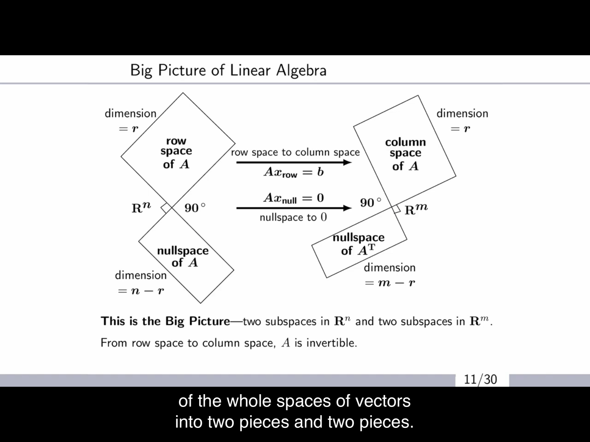
4 Subspaces

There are four major subspaces; Column space, Null space, Row space, Null space of A transpose (a.k.a the left null space). Assume there is a m by n matrix A,

\[C(A) \in \R^m\\ N(A) \in \R^n\\ C(A^T) \in \R^n\\ N(A^T) \in \R^m\]

We want to know the dimension of each space because we get a lot of information such as rank, basis during calculation of the process.

\[\begin{aligned} &dim=\#\ of\ basis\\ &dim(C(A)) = \#\ of\ piv.\ cols\ of\ A=r\\ &dim(N(A)) = \#\ of\ free\ cols\ of\ A=n-r\\ &dim(C(A^T)) = \#\ of\ piv.\ cols\ of\ A=r\\ \end{aligned}\]

What about the left null space?

\[\begin{aligned} A^T\boldsymbol{y}&=\boldsymbol{0}\\ \boldsymbol{y^T}A&=\boldsymbol{0^T}\\ row\times A&=row \end{aligned}\]

By row operation, we are able to get zero row. So, we need to know special solutions that would lead us to zero row by conducting row operation to A and we can attain this by using reduced row echelon form.

\[\begin{aligned} E\begin{bmatrix} A_{m\times n}&I_{m \times m} \end{bmatrix}\rightarrow\begin{bmatrix} R_{m \times n}&E_{m \times m} \end{bmatrix} \end{aligned}\]

So, the last rows that would transform rows of A into zero rows would be the basis and the number of it (=free rows of R) would be the dimension of the left null space.

\[\begin{aligned} dim(N(A^T))=\#\ of\ free\ rows\ of\ R\ or\ A=m-r \end{aligned}\]

These 4 subspaces are going to be essential to understand the linear relation btw solutions and matrices in next further steps.