Introduction

The note is based on a MIT open course by professor Gilbert Strang. The post is continued from the previous post

Contents

1. Matrices
2. Spaces
3. Projections
4. Orthogonality
5. Determinants
6. Eigenvalues & Eigenvectors

Projections

Intro to Projections

As we know, there are times when \(A\boldsymbol{x}=\boldsymbol{b}\) have no solution because the matrix A is very rarely full rank. In this case, we must find the best solution. One of the best solution to this problem is to project p to the column space of Q because that is the only when the solution exists.

Let us project vector b onto vector a. The new projected vector p would be some scalar x times a. \(\begin{aligned} &\boldsymbol{p}=x\boldsymbol{a}\\ &\boldsymbol{a}^T(\boldsymbol{b}-x\boldsymbol{a})=\boldsymbol{0}\\ &x\boldsymbol{a}^T\boldsymbol{a}=\boldsymbol{a}^T\boldsymbol{b}\\ &\boldsymbol{p}=\frac{\boldsymbol{a}^T\boldsymbol{b}}{\boldsymbol{a}^T\boldsymbol{a}}\boldsymbol{a}=\frac{\boldsymbol{a}\boldsymbol{a}^T}{\boldsymbol{a}^T\boldsymbol{a}}\boldsymbol{b}=P\boldsymbol{b}\\ &P:projection\ matrix \end{aligned}\)

Therefore, to project b onto a, we need to apply a projection matrix to it, just like how we conducted row operation through elemental matrix and row exchanges through permutation matrix.

Projection Matrix

There are few important properties we need to know about the projection matrix.

\[\begin{aligned} &P\boldsymbol{b}=C(P)\\ &P^T = P\\ &P^2 = P \end{aligned}\]

Noticing that the projected vector p is a vector that is in the column space of P is very important. And the difference between the vector and the projected one is called; error in letter, e. The error vector is always perpendicular to the column space of P. Let us use the figure above to understand why.

\[\begin{aligned} &\boldsymbol{e} = \boldsymbol{\hat{p}}-\boldsymbol{p}\\ &\boldsymbol{q_1}^T(\boldsymbol{\hat{p}}-\boldsymbol{p})=\boldsymbol{0}\\ &\boldsymbol{q_2}^T(\boldsymbol{\hat{p}}-\boldsymbol{p})=\boldsymbol{0}\\ &\leftrightarrow\\ &\begin{bmatrix} \boldsymbol{q_1}^T\\\boldsymbol{q_2}^T \end{bmatrix}(\boldsymbol{\hat{p}}-\boldsymbol{p})=Q^T\boldsymbol{e}=\boldsymbol{0}\\ &\boldsymbol{e} \in N(Q^T)\leftrightarrow\boldsymbol{e} \perp C(Q) \end{aligned}\]

So, the relation between the matrix A and the target vector b is like below.

Since we know what the properties of the projection matrix has, let us define in a higher dimension.

\[\begin{aligned} &A^TA\boldsymbol{\hat{x}}=A^T\boldsymbol{b}\\ &\boldsymbol{\hat{x}}=(A^TA)^{-1}A^T\boldsymbol{b}\\ &\boldsymbol{p} = A\boldsymbol{\hat{x}}=A(A^TA)^{-1}A^T\boldsymbol{b}\\ &P=A(A^TA)^{-1}A^T \end{aligned}\]

Recall from the previous post, when I was explaining why we need transpose. Transpose are mostly used to create a symmetric matrix and this is one of the most common problems where it is used.

But is \(A^TA\) always invertible? We need to remind ourselves that A is not a square invertible matrix or else it would already have a solution that exist. We wouldn’t have to go through all this complicated process. The problem for Ax is that there are just too many equations that there are “noise” which also means there are too many rows in A. So, if A doesn’t have a full row rank, what about the column rank? Let us say that A has independent columns,

\[\begin{aligned} &A^TA\boldsymbol{x}=\boldsymbol{0}\\ &\boldsymbol{x}^TA^TA\boldsymbol{x}=(A\boldsymbol{x})^T(A\boldsymbol{x})=0\\ &||A\boldsymbol{x}||^2=0\\ &A\boldsymbol{x}=\boldsymbol{0}, x=\boldsymbol{0}\\ &\therefore A^TA\boldsymbol{x}=\boldsymbol{0}, x=\boldsymbol{0}\\ \end{aligned}\]

we made sure in the previous post that when a matrix A has full column rank (r=n), x must be a zero vector. So, \(A^TA\) also has no free columns just the pivots which proves that it is invertible.

Orthogonality

Intro to Orthogonality

Coming back to the 4 subspaces,

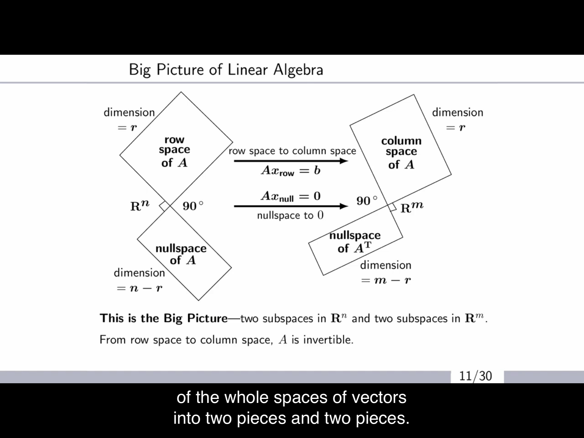
we are going to try and understand,

\[\begin{aligned} C(A) \perp N(A^T)\\ C(A^T) \perp N(A) \end{aligned}\]

When we say two subspaces are orthogonal to each other, do we mean that the every vector from each space is orthogonal to each other? No, because we have the intersection space and the zero vector.

Think of \(A\boldsymbol{x}=\boldsymbol{0}\),

\[\begin{aligned} &\begin{bmatrix} row1\ of\ A\\ row2\ of\ A\\ .\\ .\\ .\\ rown\ of\ A\\ \end{bmatrix}\begin{bmatrix} x_1\\x_2\\.\\.\\.\\x_n \end{bmatrix}=\begin{bmatrix} 0\\0\\.\\.\\.\\0 \end{bmatrix}\\ &\rightarrow (combination\ of\ rows\ of\ A)^T\boldsymbol{x}=\boldsymbol{0}\\ &\leftrightarrow N(A) \perp C(A^T) \end{aligned}\]

and since the sum of their dimension is the whole dimension, the two spaces are called the complements of space $\R^n$. In other words, the null space contains all vectors perpendicular to the row space. Additionally, by the equation above, this also means all vectors in null space is linearly independent to the vectors in row space.

\(\begin{aligned} &N(A) \perp C(A^T) &\rightarrow N(A), C(A^T)\ are\ linearly\ independent \end{aligned}\)

Orthogonal Matrix

When there are unit vectors that are perpendicular to each other we call them; orthonormal vectors. When a matrix with these as columns; orthonormal matrix is squared, we call them; Orthogonal matrix. These are super useful,

\[\begin{aligned} &Q^TQ = QQ^T = I\\ &Q^T = Q^{-1}\\ &Q: orthogonal;\ square;\ invertible \end{aligned}\]

Think of the projection matrix. If the matrix A has orthonormal columns, the equation becomes a lot more eaiser.

\[\begin{aligned} &A=\begin{bmatrix} q_1&q_2&\cdots& q_n \end{bmatrix}\\ &P = A(A^TA)^{-1}A^T = AA^T\\ &A^TA\hat{x}=A^Tb \leftrightarrow \hat{x}_i=q_i^Tb \end{aligned}\]

Gram-Schmidt is a very useful way to make these matrices.

Gram-Schmidt

The goal of Elimination was to try and make a triangular matrices because we need them for figuring out solutions i.e. pivots; ranks. The goal of Gram-Schmidt is to make orthogonal matrices.

The first step is to make two orthogonal vectors and then make them into unit vectors.

\[\begin{aligned} &two\ independent\ vectors\ a_1, a_2\\ &u_1=a_1\\ &u_2=a_2-\frac{a_1a_1^T}{a_1^Ta_1}a_2\\ &u_1^Tu_2=0\\ &q_1=\frac{u_1}{||u_1||},q_2=\frac{u_2}{||u_2||} \end{aligned}\] \[\begin{aligned} &three\ independent\ vectors\ a_1,a_2,a_3\\ &u_1=a_1\\ &u_2=a_2-\frac{a_1a_1^T}{a_1^Ta_1}a_2\\ &u_3=a_3-\frac{a_2a_2^T}{a_2^Ta_2}a_3-\frac{a_1a_1^T}{a_1^Ta_1}a_3\\ &u_3 \perp a_2, u_3 \perp a_1\\ &!\ u_2\ not\ perpedicular\ to\ a_3 \end{aligned}\]

Therefore, the process of making orthonormal vectors is just a combination of the column vectors. So the matrix that has column a and b has the same column space with the orthogonal matrix.

\[\begin{aligned} &A?=Q\\ &\begin{bmatrix} a_1&a_2&\cdots&a_n \end{bmatrix}\begin{bmatrix} & \ & \\ & ? & \ \\ \ & \ \\ \end{bmatrix}=\begin{bmatrix} q_1&q_2&\cdots&q_n \end{bmatrix}\\ &\leftrightarrow\\ &Q^{-1}A=Q^TA=\begin{bmatrix} q_1^T\\q_2^T\\ \vdots \\ q_n^T \end{bmatrix}\begin{bmatrix} a_1&a_2&\cdots&a_n \end{bmatrix}=\begin{bmatrix} q_1^Ta_1&q_1^Ta_2&\cdots&q_1^Ta_n\\ 0&\ddots&\ &\vdots\\ \vdots&\ &\ddots&\vdots\\ 0&\cdots&\cdots&q_n^Ta_n\\ \end{bmatrix}\\ &\therefore A=QR\\ &R: upper\ triangular\ matrix \end{aligned}\]