Introduction

The note is based on a MIT open course by professor Gilbert Strang. The post is continued from the previous post

Contents

1. Matrices
2. Spaces
3. Projections
4. Orthogonality
5. Determinants
6. Eigenvalues & Eigenvectors

Determinants

Properties

Before looking at the formula, we need to understand the 10 properties (especially the top 3) of determinants.

1) det(I)=1

2) Exchange rows: reverse sign of det

\(\begin{aligned} det(P) = 1\ or\ -1 \end{aligned}\)
If the number of exchange is even; 1, odd; -1.

3) determinant is linear in each seperate row

\(\begin{aligned} &\begin{vmatrix} ta&tb\\c&d \end{vmatrix}=t\begin{vmatrix} a&b\\c&d \end{vmatrix}\\ &\begin{vmatrix} a+a'&b+b'\\c&d \end{vmatrix}=\begin{vmatrix} a&b\\c&d \end{vmatrix}+\begin{vmatrix} a'&b'\\c&d \end{vmatrix} \end{aligned}\)

4) 2 equal rows; det=0

Use property 2. Exchanging row should change the sign.

5) det(A)=det(U)

Subtract l row i from row k doesn’t change the determinant. Use property 3 and 4 to prove it.

\[\begin{aligned} \begin{vmatrix} a&b\\c&d \end{vmatrix}=\begin{vmatrix} a&b\\c-la&d-lb \end{vmatrix}=\begin{vmatrix} a&b\\c&d \end{vmatrix}-l\begin{vmatrix} a&b\\a&b \end{vmatrix} \end{aligned}\]

6) rows of zeros; det=0

Use property 3 to prove it.

\[\begin{aligned} 0\begin{vmatrix} a&b\\c&d \end{vmatrix}=\begin{vmatrix} 0&0\\c&d \end{vmatrix} \end{aligned}\]

7) det=product of pivots

We learned that we can transform any matrix into a diagonal one by elimination and permutation. Additionally, by property 3, the determinant of diagonal matrix is the product of diagonal elements and the determinant of identity matrix.

\[\begin{aligned} det(A)=det(D)=d_nd_1\cdots d_1det(I) \end{aligned}\]

We have to watch out for signs and also for a zero diagonal element; free variable; singular matrix.

8) det(A)=0; singular: test for invertibility

If A is singular, row of zeroes exist after elimination. We can think about this in property 7 as well.

9) det(AB) = det(A)det(B)

\(\begin{aligned} &det(A^{-1})=\frac{1}{det(A)}\\ &det(A^{2})=det(A)^2\\ &!\ det(2A)=2^ndet(A) (\because prop\ 3) \end{aligned}\)

10) det(A) = det(A^T)

If A has zero column vector, the determinant is zero; singular matrix.

Formula

\(\begin{aligned} &\begin{vmatrix} a&b\\c&d \end{vmatrix}=\begin{vmatrix} a&0\\c&d \end{vmatrix}+\begin{vmatrix} 0&b\\c&d \end{vmatrix}\cdots(1)\\ &=\begin{vmatrix} a&0\\c&0 \end{vmatrix}+\begin{vmatrix} a&0\\0&d \end{vmatrix}+\begin{vmatrix} 0&b\\c&0 \end{vmatrix}+\begin{vmatrix} 0&b\\0&d \end{vmatrix}\cdots(2)\\ &=\begin{vmatrix} a&0\\0&d \end{vmatrix}-\begin{vmatrix} c&0\\0&b \end{vmatrix}\cdots(3)\\ &=ad-bc\\ &\begin{vmatrix} a&b\\c&d \end{vmatrix}=\begin{vmatrix} a&b\\0&d \end{vmatrix}+\begin{vmatrix} 0&b\\c&d \end{vmatrix}\cdots(4) \end{aligned}\)

We can understand the formula just by reviewing the property. (1) First, seperate the matrix by the first row. (2) Next, split the seperated matrices by the second row. Notice the matrices with zero column that can be crossed out. (3) Lastly, manage the sign. So, basically, the formula of the determinant is the multiplication of the diagonal elements of linearly seperated diagonal matrices. The key point in this process is to cross out the matrix with zero column vector or row vector. (4) By property 10, I don’t see why not we can’t split the matrix by columns. In conclusion, we can organize our thoughts like below.

\[\begin{aligned} &\begin{vmatrix} r_1\\r_2\\\vdots\\r_n \end{vmatrix} \rightarrow \sum\plusmn\begin{vmatrix} a_{1a}\\ \ &a_{2b}\\ \ & \ & \ddots\\ \ & \ & \ & a_{nw} \end{vmatrix}\cdots(1)\\ &(a,b, \cdots w) = permutation\ of\ 1, \cdots n\\ \\ &\begin{vmatrix} a_{11}& \cdots & \ \\ \vdots & \ & \ \\ & \ & \ \end{vmatrix} \rightarrow \begin{vmatrix} a_{11}& 0 & 0 \\ 0 & A_2 & \ \\0 & \ & \ \end{vmatrix} \rightarrow a_{11}|A_2|\cdots(2) \end{aligned}\]

(1) The matrix would be seperated by row until there is one none zero element in the pivot row. Again, the next row becomes the next pivot. By the time we are done with all the rows there must be matrices with zero column vectors which will be all crossed out. Then each row would only have nonzero elements that can be shifted into diagonal matrix; product of pivots. (2) What we did in mind in (1) is operating only with pivot rows. To make the diagonal matrix, it means that each column also has only one pivot element. So, there would be much more less calculation if we choose the pivot row and column same time. Therefore, not focusing row by row, if we focus determinant by determinant it would be 2^n as faster.

Coming back to the idea (1) the formula would be,
\(det A = \sum \plusmn a_{1a}a_{2b}\cdots a_{nw}\)

Cofactor

Since we know how the determinant works, it would be nice if we can write this in algebra.

\[\begin{aligned} &|A| = a_{11}|A_{n-1}^1|+a_{12}|A_{n-1}^2|+\cdots+a_{1n}|A_{n-1}^n|\\ &=a_{11}C_{11}+a_{12}C_{12}+\cdots+a_{1n}C_{1n}\\ &C_{ij} = \plusmn det\ of\ n-1\ matrix\ with\ row\ i\ col\ j\ erased\\ &+: i+j\ even,\ -: i+j\ odd \end{aligned}\]

Going back to idea (2), when a pivot is selected, the first part of the matrix can be seperated as given. All it needs is the next corresponding determinant; cofactor.

Formula for Inverse

\(\begin{aligned} &A^{-1}=\frac{1}{detA}C^T\\ &C=\begin{bmatrix} C_{11}&\cdots& C_{1n}\\ \vdots & \ & \vdots\\C_{n1}&\cdots&C_{nn} \end{bmatrix}\\ &AC^T=(detA)I\\ &\because a_{i1}C_{j1}+\cdots a_{in}C_{jn}=0 \cdots(1) \end{aligned}\)

Think about the formula of determinant again. It’s the sum of pivot element multiplied by the corresponding n-1 matrix with the same row and column erased. In case of (1), this is when the cofactor is not corresponding to the pivot element. In other words, it is when the pivot element has either non zero element in its row or column; det=0.

Cramer’s Rule

\(\begin{aligned} &Ax=b\\ &x=A^{-1}b=\frac{1}{detA}C^Tb\\ &C^Tb=C_{1i}b_{1}+\cdots+C_{ni}b_{n}: det\ of\ some\ (matrix)_i\\ &x_1=\frac{detB_1}{detA}\\ &x_2=\frac{detB_2}{detA}\\ \end{aligned}\)

Cramer found out what the matrix B is.
\(\begin{aligned} &B_1=\begin{bmatrix} b&A_{n-1} \end{bmatrix}=\begin{bmatrix} A\ with\ col1\ replaced\ by\ b \end{bmatrix}\\ &detB_1=b_1C_{11}+\cdots \end{aligned}\)
However, this doesn’t really solve the problem since there is the need for too much calculation.

Det gives Volume

This is the most essential part of this chapter. The determinant of a matrix can give us the volume of a box with coordinates.

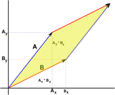
The determinant of a matrix that has vector A and B as column vector is equal to the size of the parallelogram. This enables us to attain a volume of a figure without knowing the length or angles. The volume has the same property as the determinant does.

Eigenvalues & Eigenvectors

Intro to eigenvectors and values

Eigenvectors are special vectors that are parellel to when multiplied with A.

\[\begin{aligned} &Ax=\lambda x, x\neq0\\ &x: eigenvector\\ &\lambda: eigenvalue \end{aligned}\]

It is when this special vector is on the column space of A. So, if the matrix A is singular, one of the eigenvalues must be zero since there is at least more than one eigenvector in its null space. Also, if we think about the orthogonality of these vectors, they are perpendicular to each other.

The eigenvalues and eigenvectors are very much useful as much as rank and dimension is to understand a matrix.

How to solve

\(\begin{aligned} &Ax=\lambda x\\ &(A-\lambda I)x=0, x\neq0\\ &singular \leftrightarrow det(A-\lambda I)=0 \end{aligned}\)

If we move the right side of the equation to the left, we can see that it is a singular matrix which is solvable by the determinant. Then we are able to find eigenvalues and the corresponding eigenvectors.

An interesting property about the eigenvalues and eigenvectors can be seen below,

\[\begin{aligned} Bx=(A+3I)x=\lambda x + 3x \end{aligned}\]

The new matrix B has same eigenvectors as A does. So there must be something with the diagonal elements.

Useful Properties

\(\begin{aligned} &trace=\sum\lambda\\ &det=\prod\lambda \end{aligned}\)

Matrices with problems

1. Matrices w/ problems in eigenvalues

   Rotation matrices have complex eigenvalues. These matrices are antisymmetic (Q^T=-Q). In contrast, symmetric matrices have real eigenvalues.

2. Matrices w/ problems in eigenvectors

   Triangular matrices have insufficient eigenvectors because at least one of its column vectors of \(A-\lambda I\) is a zero column.

These matrices are considered “not good”. They all have purpose, but they are not always best because they might not be “good” enough for later process. This is why we need to define and find “good” matrices.

Diagonalizing a matrix

Suppose that there are n independent eigenvectors of A, and let us put them in columns of a matrix S.

\[\begin{aligned} AS &= A\begin{bmatrix} x_1&x_2&\cdots&x_n \end{bmatrix}=\begin{bmatrix} \lambda_1 x_1&\lambda_2 x_2&\cdots&\lambda_n x_n \end{bmatrix}\\ &=\begin{bmatrix} x_1&x_2&\cdots&x_n \end{bmatrix}\begin{bmatrix} \lambda_1&0&\cdots&0\\0&\ddots& \ \\ \vdots & \ & \ddots & \\\ 0& \ & \ &\lambda_n \end{bmatrix}=S\Lambda\\ &\leftrightarrow A=S\Lambda S^{-1} \end{aligned}\]

This is called diagonalization; factoring the matrix A into eigenvectors units. Additionally, ince the eigenvectors are perpendicular to each other, it would be very nice if it was orthonormal as well. This will be covered shortly later.

This factorization gives us a good sense of what powers of matrix is.

\[\begin{aligned} &A^2x=\lambda^2x\\ &A^2=S\Lambda S^{-1}S\Lambda S^{-1}=S\Lambda^2S^{-1}\\ &A^k = S\Lambda^k S^{-1} \end{aligned}\]

Differential Equation & Matrix Exponential

Differential Equation

A differential equation is a mathematical equation for an unknown function of one or several variables that relates the values of the function itself and of its derivatives of various orders. A matrix differential equation contains more than one function stacked into vector form with a matrix relating the functions to their derivatives. Let say, for example we’re to find what u(t) is.

\[\begin{aligned} &\frac{du_1}{dt}=-u_1+2u_2\\ &\frac{du_2}{dt}=u_1-2u_2\\ &given\ u(0)=\begin{bmatrix} 1\\0 \end{bmatrix}\\ \rightarrow&\frac{du}{dt}=\begin{bmatrix} -1&2\\1&-2 \end{bmatrix}u=Au \end{aligned}\]

The solution for the u(t) is as below,

\[\begin{aligned} solution: u(t)=c_1e^{\lambda_1t}x_1+c_2e^{\lambda_2t}x_2 \end{aligned}\]

An additional comment about what u(t) is: it is a nx1 vector of functions of an underlying t.

So, we need to find what the eigenvalues and the eigenvectors are. Luckily, we see that the matrix A is singular, so the eigenvalues are very simple. Once we attain them, we can input the given t and attain the unknown scalars.

\[\begin{aligned} &\lambda=0,3\\ &x_1=\begin{bmatrix} 2\\1 \end{bmatrix},x_2=\begin{bmatrix} 1\\-1 \end{bmatrix}\\ &u(0)=\begin{bmatrix} 2&1\\1&-1 \end{bmatrix}\begin{bmatrix} c_1\\c_2 \end{bmatrix}=Sc=\begin{bmatrix} 1\\0 \end{bmatrix}\\ &u(t)=\frac{1}{3}\begin{bmatrix} 2\\1 \end{bmatrix}+\frac{1}{3}e^{-3t}\begin{bmatrix} 1\\-1 \end{bmatrix} \end{aligned}\]

Something we can notice about this vector of functions is that it is a steady state. When t is approaching infitnite, the vector is always in the same direction.

\[\begin{aligned} u(\infin)=\frac{1}{3}\begin{bmatrix} 2\\1 \end{bmatrix} \end{aligned}\]

There are three types of stability in total: zero vector, steady, blow-up.

\[\begin{aligned} &u(t) \rightarrow 0: all \lambda<0, \lambda \in C \cup Re\\ &u(t) \rightarrow cv: \lambda\leq0, \lambda \in Re\\ &u(t) \rightarrow \infin: any\ \lambda>0, \lambda \in Re\\ \end{aligned}\]

Coming back to the solution, we’re going to write the equation in the matrix S and lambda. Currently, the vector u is coupled with A, we will uncouple (diagonalizing) it to see a better picture. The whole point of eigenvectors is to uncouple a matrix.

\[\begin{aligned} &\frac{du}{dt}=Au\\ &u=Sv, S:eigenvectors\ of\ A\\ &S\frac{dv}{dt}=ASv\\ &\frac{dv}{dt}=S^{-1}ASv=\Lambda v\\ &notation:v(t)=e^{\Lambda t}v(0)\\ &(\because\frac{dv_1}{dt}=\lambda_1v_1)\\ &\therefore u(t)=Se^{\Lambda t}S^{-1}u(0)\\ \end{aligned}\]

Matrix Exponential

What does matrix exponential mean? Let us look how it was formed. Coming back to the differential equation solution above,

\[\begin{aligned} &u(t)=Se^{\Lambda t}S^{-1}u(0)\\ &e^{At}=Se^{\Lambda t}S^{-1}\\ &since,\\ &e^{At}=I+At+\frac{(At)^2}{2!}+\frac{(At)^3}{3!}+\cdots+\frac{(At)^n}{n!}+\cdots\\ &(\because taylor\ theorem)\\ &\therefore e^{At}=I+\frac{Se^{\Lambda t}S^{-1}}{2}t^2+\frac{Se^{\Lambda t}S^{-1}}{6}t^3+\cdots\\ &=S(I+\Lambda t +\frac{\Lambda^2}{2}t^2+\cdots)S^{-1}=Se^{\Lambda t}S^{-1} \end{aligned}\]

Now, does this work the whole time? Assumption: A can be diagonalized which means that A has to be one of the “good” matrices. To conclude, how do we express the matrix exponential?

\[\begin{aligned} \Lambda&=diag(\lambda_i)\\ e^{\Lambda t}&=diag(e^{\lambda_it}) \end{aligned}\]

Symmetric Matrices & Positive Definite Matrices

One of the “bad” matrices is when a matrix has complex eigenvalues. The symmetric matrices only have real eigenvalues. Another reason why these matrices are special is because the eigenvectors are orthonormal. So, this will be our definition of “good” matrices and we’ll learn how to use them.

\[\begin{aligned} &\overline{a+ib}=a-ib\\ &Ax=\lambda x\\ &A\overline{x}=\overline{\lambda x}\\ &\overline{x}^TA=\overline{x}^T\overline{\lambda} (\because A=A^T)\\ &\overline{x}^TAx=\overline{x}^T\overline{\lambda}x\\ &\overline{\lambda}=\lambda \in Re \cdots(1)\\ \\ &A^TA=A^2=S\Lambda^2 S^{-1}(\because A=A^T)\\ &\Lambda S^TS\Lambda S^TS=S^TS\Lambda^2\\ &\Lambda S^TS=\Lambda\\ &S^TS=I\\ &S^T=S^{-1}\cdots(2)\\ \\ \therefore&A=Q\Lambda Q^T \end{aligned}\]

Additionally, there are matrices that are better, and we’ll call them “excellent”. Coming back to the determinant,

\[\begin{aligned} &A=A^T\\ &det(A)=\prod diag(A) = \prod \lambda\\ &\leftrightarrow \#\ pos\ pivots\ = \#\ pos\ \lambda's \end{aligned}\]

Symmetric matrices with positive eigenvalues; Positive Definite Symmetric Matrices have positive pivots. This also means, all its subdeterminants are positive, so, we don’t have to think about the sign of cofactors.

But how doe we know that a matrix is a positive definite? There are four tests in total.

1. eigenvalues > 0
2. determinant > 0
3. pivots > 0
4. \[x^TAx > 0, x \neq 0\]

Any of them is fine, but the 4th is the most important. The rest is good but not the best. Let us think of an example.

\[\begin{aligned} &given\ A=\begin{bmatrix} 2&6\\6&20 \end{bmatrix},\\ &x^TAx=2x_1^2+20x_2^2+12x_1x_2 > 0 \end{aligned}\]

The equation above is a quadratic form. We need to figure out whether the form is positive or not.

\[\begin{aligned} &x^TAx=2x_1^2+20x_2^2+12x_1x_2\\ &=2(x_1+3x_2)^2+2x_2^2>0\cdots(1)\\ &\begin{bmatrix} 2&6\\6&20 \end{bmatrix}\rightarrow\begin{bmatrix} 2&6\\0&2 \end{bmatrix}\rightarrow\begin{bmatrix} 2\sdot1&2\sdot3\\0&2 \end{bmatrix}\cdots(2) \end{aligned}\]

The form (1) certains that the form is above zero. This can be attained easily if we implement elimination. When this quadratic surface is shown in geometry in higher dimension, it will mostly look like below. In this case, would be the elliptic paraboloid.

How can we generate positive definited matrices? This when the quadratic form shines. Given m by n matrix with full column rank; no null space,

\[\begin{aligned} &A^TA: pos.\ def\\ &x^T(A^TA)x=||Ax||^2>0 \end{aligned}\]

Similar Matrices

When we say two matrices such as A and B are similar, it means that B can express A like below,

\[\begin{aligned} B=M^{-1}AM \end{aligned}\]

An easiest example of this would be the diagonlization.

\[\begin{aligned} S^{-1}AS=\Lambda \end{aligned}\]

Why would we call A and B similar? It is because their eigenvalues are the same, but not the eigenvectors.

\[\begin{aligned} &Ax=\lambda x\\ &M^{-1}AMM^{-1}x=\lambda M^{-1}x\\ &BM^{-1}x=\lambda M^{-1}x \end{aligned}\]

Singular Value Decomposition

Now, this part is where we bring everything we’ve learned. Any matrix A that can be decomposed into three matrices. Something we have to remind ourselves,

\[\begin{aligned} A=S\Lambda S^{-1}\\ A=Q\Lambda Q^T \end{aligned}\]

When the matrix A is a positive definite matrix, the ordinary S becomes orthogonal and the ordinary lambda becomes positive. How do we factor an ordinary matrix A into orthogonal and diagonal matrices?

Since we know that the matrix is a linear mapping of vectors from a row space to a column space, or in another direction, we now understand the expression below,

\[\begin{aligned} &A_{m\times n}:R^m\rightarrow R^n\\ &v \in C(A^T), u \in C(A)\\ &v_i \perp v_j, u_i \perp u_j, ||v||,||u||=1\\ &cu=Av\\ &A\begin{bmatrix} v_1&v_2&\cdots&v_r \end{bmatrix}=\begin{bmatrix} \sigma_1u_1&\sigma_2u_2&\cdots&\sigma_nu_r \end{bmatrix}\\ &=\begin{bmatrix} u_1&u_2&\cdots&u_r \end{bmatrix}\begin{bmatrix} \sigma_1& \ & \\\ \ & \ddots & \\\ \ & \ & \sigma_r \end{bmatrix}(rank(A)=r)\\ &\therefore A=U\Sigma V^T \end{aligned}\]

However, this is quite difficult to find since we have to find orthogonal bases in the rowspace that is also orthogonal in the column space after its mapping. We can find each of the bases if we understand the equation below.

\[\begin{aligned} &A^TA=V\Sigma^T\Sigma V^T\\ &AA^T=U\Sigma^T\Sigma U^T\\ \end{aligned}\]

We can see that the matrices V & U are the eigenvector matrices of each of the positive symmetric matrix.